How to Freeze Rows and Columns in Google Sheets

Your header rows disappear when you scroll down through your data in Google Sheets. You can keep those specific rows and columns locked in place while you navigate your spreadsheet.

1. Select the row you want to lock, right-click it, go to “View more row actions,” and select “Freeze up to row [number].” [0:12]
2. To lock multiple rows, select the bottom row of your desired range, right-click, and choose the freeze option for that row. [0:41]
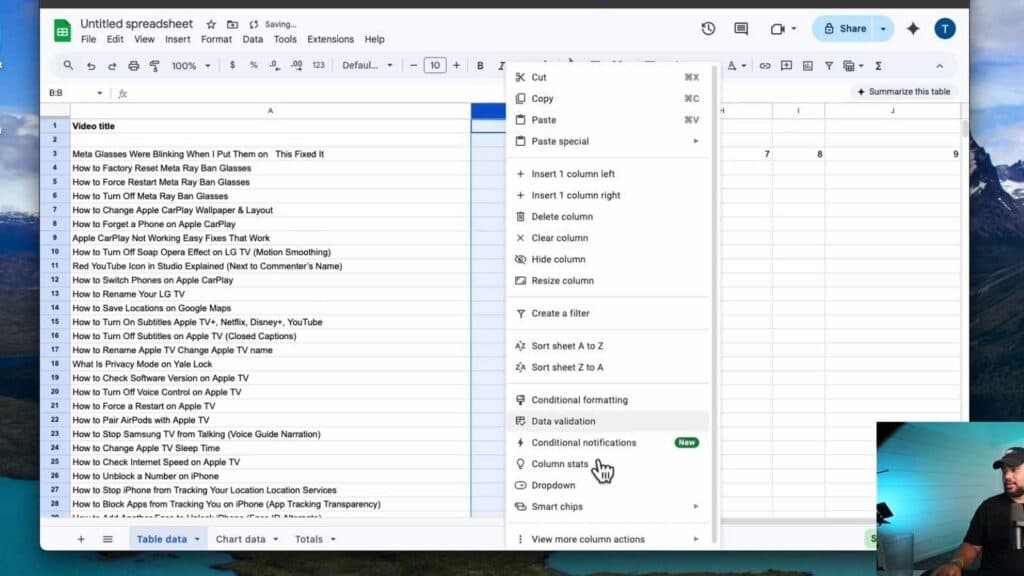
3. If you need to lock columns, select the column you want to freeze, right-click, and choose “Freeze up to column [letter].” [1:37]
4. You can combine these methods to freeze both your header rows and your sidebar columns at the same time. [2:09]
5. To remove these locks, go to the “View” menu, select “Freeze,” and choose “No rows” or “No columns” to return your sheet to its original state.

Ninja Tip: You can also drag the thick gray lines located at the top-left corner of the grid area to manually adjust your frozen rows or columns without using the menu at all.

If your sheet remains unresponsive or displays formatting errors, go to Help > Clear cache and refresh the page.