How to Create and Color-Code Drop-Down Lists in Google Sheets

Your Google Sheet currently lacks a structured way to select data, which slows down your workflow. You can easily fix this by creating custom drop-down lists with specific color-coded options.

1. Select the range of cells where you want your drop-down list to appear and click Data followed by Data validation [0:25].
2. Click Add rule and choose whether to manually type in your values or pull them from an existing range in your sheet [0:43].
3. Assign a specific color to each of your list items within the validation menu to keep your data organized [1:41].
4. Expand the Advanced options menu to switch your display style between chips, arrows, or plain text [2:26].
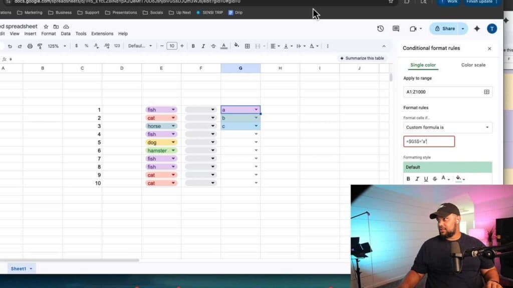
5. To make an entire row change color based on your selection, select your data range and navigate to Format then Conditional formatting [3:10].
6. Under the Format rules section, select Custom formula is and enter your formula, such as = $G5 = "A", to apply a color to the row when that specific option is chosen.
7. Repeat the conditional formatting process for every unique item in your drop-down list to ensure every category has its own distinct row color.

Ninja Tip: You can quickly add a secondary drop-down that changes based on your first selection by using the INDIRECT function combined with named ranges to create dependent lists.

If you need to revert your sheet to its original state, go to File > Version history > See version history.